In biology a blind pan is a powerful technique that allows you to obtain ligands for structures that are not well characterized, as well as bypass issues like protein denaturation that plague typical pans against a purified protein target bound to a plate.
Pros:
- Does not require any knowledge of a structure’s proteome characteristics to work
- Ligands are introduced to proteins in a more natural conformation
- Reduces chances of epitope blocking
Cons:
- Finding the receptor your ligand targets is often challenging
However the main problem with a blind pan is in the name, its blind. This means that even if your pan spits out a functional peptide, you don’t know what your peptide is interacting with to achieve its function.
One common way to find the receptor is using a guided covalent pulldown, where the ligand from the blind pan is attached to a scaffold that contains an oxime or similar group that will form a covalent bond with a nearby protein. This scaffold is incubated with cell lysate then a digestive agent is added to break apart the proteins into fragments. The fragments bound to the scaffold are separated to determine which protein the most common fragments belong to. The problem though is that most likely hits are determined only by the protein that had the most fragments show up in the data. This method of quantification does not work well given that this assay has a poor signal to noise ratio, covalent pulldowns bind irrelevant proteins, plastic fragments, and other compounds that muddy the data.
I built covalent pocket mapper in an effort to solve that. Covalent pocket mapper is a tool that accounts for the chemical and physical properties of your scaffold, and is built on the assumption that the protein fragments bound through true peptide interaction (the signal) will be centered around a given binding pocket, whereas protein fragments from contaminants (noise) should be randomly distributed across the exposed protein surface. The first thing the tool needs is an honest model of how far your scaffold can actually reach. Typically the scaffold is a flexible polymer, so its reach is not a single length but a distribution, P(r), the probability that its two ends sit a distance r apart. Covalent pocket mapper derives that from chemistry from the backbone bonds of your repeat unit: the bond length and angle, and how the bond twists. An ordinary single bond is a rotational-isomeric-state bond and wants rotamer energies from a polymer reference, while a double bond, amide, or aromatic bond is simply rigid. Those rotamer energies become Boltzmann weights, so a 0.5 kcal/mol gauche penalty makes the trans state roughly 2.3× more likely at room temperature and stiffens the chain, whereas PEG’s O–C–C–O gauche effect runs the other way and makes it curl. The tool then grows ~120,000 copies of the chain and records where each one ends up. PEG8 has a fully-stretched length of 28.9 Å, but its most likely end-to-end distance is only 10.6 Å. If you can’t find rotamer energies for your polymer, you can skip the form and give a persistence length instead, which is tabulated for essentially everything common.
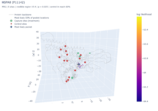
With P(r) in hand the geometry becomes straightforward. Each captured fragment tells you one end of the scaffold was covalently pinned to a specific atom, so the reach model becomes a cloud of probability in the space around that atom — dense where the free end most likely landed, thinning inward and outward, and exactly zero past the contour length. Every capture site casts its own cloud, and the tool multiplies them together. Because the density is genuinely zero beyond the chain’s physical limit, a single site the scaffold could not have reached rules out that location no matter how well every other site agrees. The search runs over the solvent shell just outside the protein, since a covalent partner has to be reachable, and the peak of the combined cloud is the inferred pocket.
For each protein you get the pocket’s coordinates in the frame of its own structure, the probability at that point, and a region saying how tightly the data actually pin it down. Significance comes from a permutation test that asks how often the same number of capture sites scattered anywhere on that protein’s surface would be explained this well by a single pocket. On my own dataset with a PEG8 scaffold, 13 of 26 proteins had any surface point reachable from all their capture sites at all, eliminating typically sticky non-specific contaminants like vimentin, filamin, talin, and tropomyosin even though all those proteins had plenty of fragments.
A negative control such as a scrambled peptide is optional but valuable here, one spurious capture site can veto a real binder, and a non-guided control serves to counter that issue.
Limitations. The N-terminus of a detected fragment is a proxy for the attachment site, your specific choice of covalent agent (oximes, acrylamides, epoxides, etc) will have an impact on the precise part of the fragment your scaffold bound to. The method needs a predicted structure and at minimum four capture sites within the modelled region, which long disordered proteins can fail. It assumes one pocket per protein, so a genuine two-site binder will usually return nothing rather than either site (I plan on addressing this in the future). And the reach model treats the scaffold as a free chain, so it doesn’t know the protein is in the way — a path that would have to tunnel through the protein still counts as reachable. This program also cannot account for any proteins that strayed from their typical conformation due to non-physiological conditions in the blind pan or guided pulldown. None of these are fatal, but they emphasize that this narrows a contaminated hit list to a small number of structurally plausible candidates with coordinates you can go and look at. If your goal is to identify a protein target for your ligand, this tool is best used as a data filtering step to obtain a short list of binding sites to perform more sophisticated docking analysis via tools like HADDOCK.